Model Optimization is the heaviest domain on the NCP-GENL exam at 17% of total weight. It is also the domain most responsible for candidate failures. The questions are scenario-heavy, requiring you to select specific optimization strategies given hardware constraints, latency requirements, and accuracy thresholds. Memorizing definitions is not enough. You need to understand the trade-offs well enough to make production-grade decisions under time pressure.
This guide covers every optimization technique tested on the NCP-GENL exam, with the formulas, trade-offs, and decision frameworks you need to answer questions correctly.
Navigation
This article focuses on the Model Optimization domain (17%). For other NCP-GENL topics:
Why Model Optimization Is the Make-or-Break Domain
At 17%, Model Optimization contributes approximately 10-12 questions to the exam. These questions are among the most technically demanding because they combine multiple concepts: you might need to calculate memory savings from quantization, then determine whether the resulting accuracy loss is acceptable for a specific use case, then select the right TensorRT-LLM configuration to meet a latency SLA.
Exam Reality Check
Model Optimization questions are rarely straightforward. A typical question provides a production scenario (model size, GPU hardware, latency requirements, accuracy constraints) and asks you to select the optimization strategy that satisfies all constraints simultaneously. You need to perform mental math quickly — knowing that a 70B model in FP16 requires ~140GB of GPU memory is the kind of instant recall the exam expects.
Run FP16 → INT8 → INT4 on a real model
This is the highest-failure domain on NCP-GENL. Quantize a real model with bitsandbytes, benchmark the memory/latency delta with precision sweep, then serve optimized with vLLM — the exam's trickiest scenarios get trivial once you've seen the numbers.
- Open labQuantize & Optimize LLMs with bitsandbytesintermediate 40 minGPU sandbox
- Open labBatch Size & Precision Sweep: Finding Your Sweet Spotintermediate 40 minGPU sandbox
- Open labvLLM Production Serving: PagedAttention, Continuous Batching, Prefix Cachingadvanced 55 minGPU sandbox
- Open labInference Serving Patterns: Dynamic Batching, Throughput, and the Triton Mental Modelintermediate 40 minGPU sandbox
- Open labProfile PyTorch Training with the Built-in Profilerintermediate 35 minGPU sandbox
Preparing for NCP-GENL? Practice with 455+ exam questions
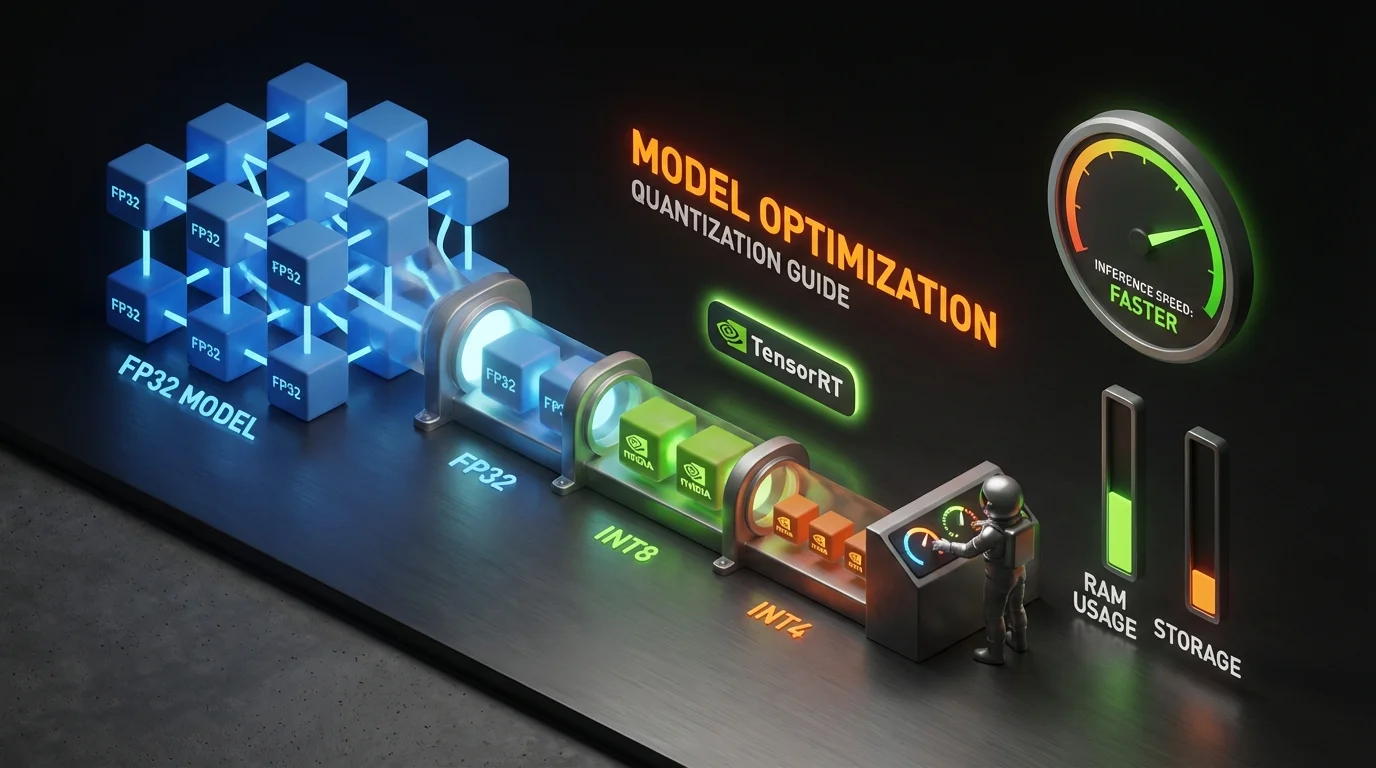
Quantization: The Core Optimization Technique
Quantization reduces the numerical precision of model parameters from higher-bit representations (FP32, FP16) to lower-bit representations (INT8, INT4), directly reducing memory footprint and improving inference speed.
Precision Formats and Memory Impact
| Format | Bits per Parameter | Memory for 7B Model | Memory for 70B Model | Relative Speed | Typical Accuracy Loss |
|---|---|---|---|---|---|
| FP32 | 32 bits (4 bytes) | 28 GB | 280 GB | 1x (baseline) | None |
| FP16 / BF16 | 16 bits (2 bytes) | 14 GB | 140 GB | 1.5-2x | Minimal (<0.5%) |
| INT8 | 8 bits (1 byte) | 7 GB | 70 GB | 2-4x | Low (1-3%) |
| FP8 (E4M3/E5M2) | 8 bits (1 byte) | 7 GB | 70 GB | 2-4x | Very low (<1%) |
| INT4 / NF4 | 4 bits (0.5 bytes) | 3.5 GB | 35 GB | 3-5x | Moderate (3-5%) |
Post-Training Quantization (PTQ)
PTQ quantizes a pre-trained model without additional training. It is the fastest path to reduced model size and is the most commonly tested quantization approach on the exam.
PTQ Methods:
| Method | How It Works | When to Use | Exam Focus |
|---|---|---|---|
| Weight-Only Quantization | Quantizes weights, keeps activations in FP16 | Minimal accuracy loss is critical | Most common exam scenario |
| Weight + Activation Quantization | Quantizes both weights and activations | Maximum throughput needed | Harder to calibrate correctly |
| Dynamic Quantization | Quantizes weights statically, activations at runtime | Variable input distributions | Lower overhead than static |
| Static Quantization | Pre-calibrates both weights and activations | Known input distribution | Highest throughput |
Calibration for INT8 Quantization:
Calibration determines the optimal scaling factors for mapping FP32 values to INT8 range. The exam tests three calibration methods:
| Calibration Method | Approach | Accuracy | Speed | Best For |
|---|---|---|---|---|
| Min-Max | Uses observed min/max values | Lower | Fastest | Quick prototyping |
| Entropy (KL Divergence) | Minimizes information loss | Higher | Slower | Production deployment |
| Percentile | Uses configurable percentile bounds | Moderate | Fast | Outlier-heavy distributions |
Exam Tip: Calibration Dataset Size
The exam frequently asks about calibration dataset requirements. The standard answer: 100-1,000 representative samples that cover the expected input distribution. Too few samples produce poor scaling factors. Too many waste compute without improving quality. The calibration dataset must be representative of production traffic, not training data.
GPTQ, AWQ, and SmoothQuant
The exam tests awareness of modern quantization algorithms beyond basic PTQ:
GPTQ (Generative Pre-Trained Transformer Quantization):
- Layer-by-layer quantization using approximate second-order information (inverse Hessian)
- Achieves INT4 quantization with minimal perplexity increase
- One-shot: no iterative training required, just a calibration pass
- Commonly used for weight-only quantization of decoder-only models
AWQ (Activation-Aware Weight Quantization):
- Identifies "salient" weight channels by analyzing activation magnitudes
- Protects important weights from aggressive quantization
- Better accuracy than GPTQ at INT4 for many models
- Faster quantization process than GPTQ
SmoothQuant:
- Addresses the challenge of quantizing activations (which have outlier channels)
- Migrates quantization difficulty from activations to weights using a mathematically equivalent smoothing transformation
- Enables INT8 weight + INT8 activation quantization (W8A8) with minimal accuracy loss
- Key formula: smooths per-channel activation scales by dividing activations and multiplying weights by the same factor
Quantization Algorithm Comparison
| Algorithm | Precision | Target | Calibration | Accuracy (INT4) | Speed |
|---|---|---|---|---|---|
| GPTQ | INT4/INT3 | Weights only | 100-500 samples | Good | Minutes |
| AWQ | INT4 | Weights only | Small calibration set | Better than GPTQ | Minutes |
| SmoothQuant | INT8 W8A8 | Weights + activations | Per-channel statistics | Best for INT8 | Fast |
| Round-to-Nearest (RTN) | INT4/INT8 | Weights only | None | Worst | Instant |
FP8 Quantization on Hopper GPUs
NVIDIA Hopper architecture (H100, H200) introduces native FP8 support. This is increasingly tested on the exam:
- E4M3 (4-bit exponent, 3-bit mantissa): Higher dynamic range, used for weights and activations during forward pass
- E5M2 (5-bit exponent, 2-bit mantissa): Even higher dynamic range, used for gradients during backward pass
- FP8 provides INT8-level throughput with FP16-level accuracy because it preserves floating-point representation
- No calibration required (unlike INT8), making deployment simpler
Exam Pattern: FP8 vs INT8
When a question mentions Hopper or H100 GPUs and asks for the best quantization strategy with minimal accuracy loss, FP8 is often the correct answer. FP8 gives you INT8-level speed without the calibration complexity and with better accuracy preservation. On pre-Hopper GPUs (A100), this option does not exist — INT8 with entropy calibration is the standard.
TensorRT-LLM Optimization Pipeline
TensorRT-LLM is NVIDIA's library for optimizing and deploying LLMs with maximum inference performance. It is central to the NCP-GENL exam.
The TensorRT-LLM Optimization Workflow
Pre-trained Model (HF / PyTorch)
        │
        ▼
  1. Model Conversion
     (Convert to TensorRT-LLM format)
        │
        ▼
  2. Quantization
     (Apply INT8/FP8/INT4 with calibration)
        │
        ▼
  3. Engine Build
     (Compile optimized TRT engine for target GPU)
        │
        ▼
  4. Runtime Optimization
     (In-flight batching, KV cache management, paged attention)
        │
        ▼
  5. Deployment
     (Triton Inference Server or NVIDIA NIM)
Key TensorRT-LLM Features Tested on the Exam
In-Flight Batching (Continuous Batching): Traditional static batching waits for the longest sequence in a batch to complete before processing new requests. In-flight batching inserts new requests into the batch as soon as a sequence finishes generating. This can improve throughput by 2-3x for workloads with variable output lengths.
KV Cache Optimization: During autoregressive generation, key-value pairs from previous tokens are cached to avoid redundant computation. TensorRT-LLM manages KV cache memory efficiently:
- Paged Attention: Allocates KV cache in non-contiguous memory pages, reducing fragmentation and allowing higher batch sizes
- KV Cache Quantization: Stores cached keys/values in INT8 or FP8, reducing cache memory by 2-4x
- Multi-Block Mode: Distributes KV cache across multiple GPU memory blocks for very long sequences
Speculative Decoding: Uses a smaller draft model to generate candidate tokens, then verifies them with the full model in a single forward pass. This can improve latency by 2-3x for models where the draft model has high acceptance rates.
TensorRT-LLM Configuration for the Exam
The exam tests your ability to select the right TensorRT-LLM settings for a given scenario:
| Optimization | When to Enable | Trade-off |
|---|---|---|
| In-flight batching | Always for production LLM serving | Minimal; nearly always beneficial |
| Paged attention | Always with in-flight batching | Small overhead for page table management |
| KV cache INT8 | When GPU memory is the bottleneck | 1-2% potential quality impact on very long sequences |
| INT8 weight quantization | Latency-sensitive applications | 1-3% accuracy loss; requires calibration |
| FP8 quantization (H100+) | Hopper GPUs; best speed-accuracy trade-off | Minimal accuracy loss; no calibration needed |
| INT4 quantization | Extreme memory constraints or edge deployment | 3-5% accuracy loss; test carefully |
| Speculative decoding | When a good draft model exists | Requires draft model; not always faster |
| Tensor parallelism | Model too large for single GPU | Communication overhead between GPUs |
Pruning: Reducing Model Size
Pruning removes parameters (weights) from the model that contribute least to its output, making the model smaller and potentially faster.
Pruning Strategies
| Strategy | What It Removes | Accuracy Impact | Speedup | Exam Frequency |
|---|---|---|---|---|
| Unstructured Pruning | Individual weights (set to zero) | Low at <50% sparsity | Requires sparse hardware support | Medium |
| Structured Pruning | Entire neurons, attention heads, or layers | Higher | Direct speedup on standard GPUs | High |
| Semi-Structured Pruning (2:4) | 2 out of every 4 elements | Moderate | 2x on Ampere+ Tensor Cores | High |
NVIDIA 2:4 Structured Sparsity: Ampere and Hopper GPUs have hardware support for 2:4 sparsity (two zero elements out of every four consecutive elements). This delivers a 2x speedup on Tensor Cores with minimal accuracy loss when combined with fine-tuning after pruning.
The typical pruning workflow for the exam:
- Train a dense model to convergence
- Apply magnitude-based pruning (remove smallest weights)
- Fine-tune the pruned model for 10-20% of original training epochs
- Optionally repeat (iterative pruning for higher sparsity)
Exam Focus: Pruning + Quantization
The exam often combines pruning and quantization in a single question. The typical correct answer involves: (1) prune the model to 2:4 structured sparsity, (2) fine-tune to recover accuracy, (3) apply INT8 quantization. This combination can reduce model size by 4-8x and improve throughput by 3-4x compared to the dense FP16 baseline.
Master These Concepts with Practice
Our NCP-GENL practice bundle includes:
- 7 full practice exams (455+ questions)
- Detailed explanations for every answer
- Domain-by-domain performance tracking
30-day money-back guarantee
Knowledge Distillation
Knowledge distillation trains a smaller "student" model to mimic the outputs of a larger "teacher" model. The student learns not just the correct answers but the full probability distribution (soft targets) over the vocabulary.
Distillation Approaches
| Approach | Teacher Output Used | Student Learns | Best For |
|---|---|---|---|
| Response Distillation | Final logits / soft labels | Output distribution | General-purpose compression |
| Feature Distillation | Intermediate layer activations | Internal representations | Preserving reasoning capability |
| Attention Transfer | Attention maps | Where to focus | Tasks requiring precise attention patterns |
Distillation Temperature:
The softmax temperature parameter controls how much information the student extracts from the teacher:
When to Use Distillation vs Quantization
| Factor | Distillation | Quantization |
|---|---|---|
| Compute Cost | High (requires training) | Low (post-training) |
| Accuracy Preservation | Can exceed teacher on specific tasks | Always loses some accuracy |
| Deployment Flexibility | Produces a new architecture | Same architecture, lower precision |
| Time to Deploy | Days to weeks | Minutes to hours |
| Best For | Creating purpose-built smaller models | Optimizing existing models for serving |
Common Exam Trap
When the question asks for the fastest path to production optimization, quantization (especially TensorRT-LLM with INT8/FP8) is almost always the correct answer. Distillation is the answer when the question specifies a need to significantly reduce model architecture size (e.g., 70B to 7B) or when the scenario involves creating a model that must run on edge devices with strict hardware constraints.
Combined Optimization Pipeline
In practice, production LLM optimization combines multiple techniques. The exam tests your ability to design end-to-end optimization pipelines.
Optimization Decision Framework
NVIDIA NIM for Optimized Deployment
NVIDIA NIM (NVIDIA Inference Microservices) packages optimized models as containerized microservices with TensorRT-LLM optimizations pre-applied. The exam tests when to use NIM vs building your own TensorRT-LLM pipeline.
Use NIM when:
- Deploying standard models (Llama, Mistral, Gemma) without custom modifications
- You need fast time-to-deployment without optimization expertise
- Running on NVIDIA GPUs with standard configurations
Build custom TensorRT-LLM pipelines when:
- Deploying fine-tuned or custom-architecture models
- You need maximum control over quantization and batching parameters
- Running non-standard hardware configurations
- Your latency SLA requires precise tuning beyond NIM defaults
Practice Questions: Test Your Knowledge
These questions mirror the style and difficulty of real NCP-GENL exam questions on Model Optimization.
Question 1: A production chatbot using a 70B model on 4x A100 80GB GPUs (320GB total) has a p99 latency of 180ms. The SLA requires 100ms. Which optimization delivers the required latency reduction with minimal accuracy impact?
A) Replace with a 13B model B) Apply FP16 to INT8 quantization with entropy calibration and enable in-flight batching in TensorRT-LLM C) Apply INT4 quantization to reduce to 2x A100 GPUs D) Implement structured pruning at 50% sparsity
Answer: B. INT8 quantization provides a 2-3x latency improvement (180ms to ~60-90ms) with only 1-3% accuracy loss. In-flight batching further improves throughput under concurrent load. Option A changes the model architecture (not an optimization). Option C over-optimizes — INT4 has higher accuracy loss than needed. Option D alone is insufficient for the required latency reduction.
Question 2: You are deploying a quantized 70B model and notice significantly degraded output quality compared to the FP16 baseline. The model was quantized using round-to-nearest (RTN) INT4. What is the most likely cause and fix?
A) The calibration dataset was too small — increase to 10,000 samples B) RTN is too aggressive for INT4 — switch to GPTQ or AWQ which use second-order information to minimize quantization error C) INT4 is inherently too lossy — use INT8 instead D) The model architecture is incompatible with quantization
Answer: B. RTN (round-to-nearest) is the simplest quantization method and performs poorly at INT4 precision because it does not account for the relative importance of different weights. GPTQ uses inverse Hessian information and AWQ uses activation-aware weight selection to preserve the most important weights, significantly improving INT4 quality. Option A is wrong because RTN does not use calibration data. Option C is overly conservative. Option D is incorrect — modern LLMs are designed for quantization.
For more practice, try our NCP-GENL practice exams with 420+ scenario-based questions and detailed explanations covering all 10 exam domains.
Summary: What to Memorize for Exam Day
| Concept | Key Facts |
|---|---|
| FP32 to FP16 | 50% memory reduction, <0.5% accuracy loss |
| FP16 to INT8 | Another 50% reduction, 1-3% accuracy loss, requires calibration |
| INT8 to INT4 | Another 50% reduction, 3-5% accuracy loss, use GPTQ/AWQ not RTN |
| FP8 (Hopper only) | INT8 speed, near-FP16 accuracy, no calibration |
| TensorRT-LLM | In-flight batching + paged attention = always enable |
| Calibration | 100-1000 representative samples, entropy method for best accuracy |
| Pruning 2:4 | 2x speedup on Ampere+, needs fine-tuning after pruning |
| Distillation | For architecture changes (70B to 7B), not for quick optimization |
| NIM | Pre-optimized containers for standard models |
For the complete exam preparation strategy, see our How to Pass NCP-GENL guide and our NCP-GENL Cheat Sheet for a printable quick reference.
Ready to Pass the NCP-GENL Exam?
Join thousands who passed with Preporato practice tests