GPU Acceleration is the second-heaviest domain on the NCP-GENL exam at 14%, contributing approximately 9-10 questions. Combined with Model Optimization (17%), these two domains account for nearly a third of the entire exam. If you cannot answer questions about parallelism strategies, distributed training frameworks, and GPU memory management, passing becomes nearly impossible.
This guide covers the distributed training concepts, parallelism strategies, and GPU profiling techniques tested on the NCP-GENL exam. Every section is organized around the decision frameworks the exam expects you to apply.
Navigation
This article covers GPU Acceleration (14%). For related NCP-GENL topics:
- Model Optimization & Quantization (17% domain)
- Fine-Tuning: LoRA, QLoRA & PEFT (13% domain)
- NCP-GENL Complete Guide
- NCP-GENL Cheat Sheet
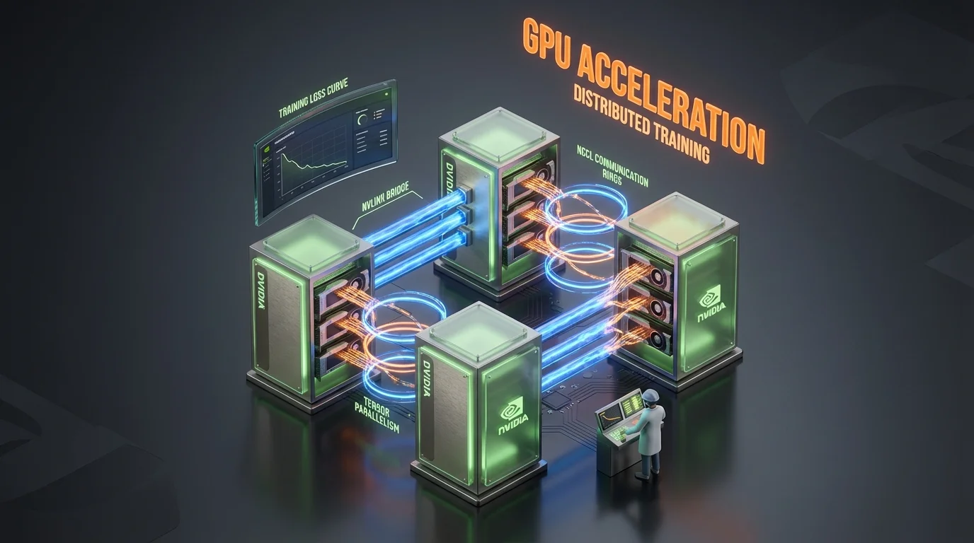
Why Models Need Distributed Training
Modern LLMs are too large to fit on a single GPU. Understanding the math behind this is foundational:
| Model Size | Memory in FP16 | Memory in FP32 | Training Memory (FP16 + Adam) | Minimum GPUs (A100 80GB) |
|---|---|---|---|---|
| 7B | 14 GB | 28 GB | ~112 GB | 2 |
| 13B | 26 GB | 52 GB | ~208 GB | 3 |
| 70B | 140 GB | 280 GB | ~1,120 GB | 14 |
| 175B | 350 GB | 700 GB | ~2,800 GB | 35 |
| 405B | 810 GB | 1,620 GB | ~6,480 GB | 81 |
Parallelism intuition from Nsight traces, not diagrams
Parallelism questions on the exam are much easier after you've watched a real Nsight trace. Profile a PyTorch training run end-to-end, see where tensor parallelism beats data parallelism, and feel the NCCL pattern differences.
- Open labNsight Systems Profiling: Finding the Bottleneck That Costs You 40% of Your GPUintermediate 35 minGPU sandbox
- Open labProfile PyTorch Training with the Built-in Profilerintermediate 35 minGPU sandbox
- Open labCUDA Programming Fundamentalsadvanced 45 minGPU sandbox
- Open labBatch Size & Precision Sweep: Finding Your Sweet Spotintermediate 40 minGPU sandbox
Preparing for NCP-GENL? Practice with 455+ exam questions
The Four Parallelism Strategies
The NCP-GENL exam tests four distinct parallelism strategies. You need to know what each does, when to use it, and the trade-offs involved.
1. Data Parallelism (DP)
How it works: Each GPU holds a complete copy of the model. The training data batch is split across GPUs, each GPU computes gradients on its data shard, and gradients are synchronized (all-reduced) across GPUs before the weight update.
GPU 0: Full Model Copy  ←→  Data Batch 0  →  Gradients 0  ╮
GPU 1: Full Model Copy  ←→  Data Batch 1  →  Gradients 1  ├→  AllReduce  →  Update
GPU 2: Full Model Copy  ←→  Data Batch 2  →  Gradients 2  ╯
When to use: The model fits entirely on a single GPU. You want to increase throughput by processing more data in parallel.
Limitations: Every GPU must hold the entire model plus optimizer states. For a 70B model in mixed precision, that is ~560GB per GPU (model + gradients + optimizer), which does not fit on any single GPU.
Communication: All-reduce of gradients after each step. Communication volume = 2 x model_size (send + receive).
2. Model Parallelism (MP) / Tensor Parallelism (TP)
How it works: Individual layers (specifically, the weight matrices within layers) are split across GPUs. Each GPU computes a portion of each layer's output, then results are combined.
Layer N Weight Matrix [4096 x 4096]
├── GPU 0: [4096 x 2048]  (left half)
└── GPU 1: [4096 x 2048]  (right half)
    → AllReduce partial results → Output
When to use: A single layer's weights are too large for one GPU, or you need to minimize per-layer latency. Tensor parallelism is most effective within a single node (intra-node) because it requires high-bandwidth communication between GPUs after every layer.
Limitations: Communication overhead after every layer. Only efficient with high-bandwidth interconnects (NVLink: 600-900 GB/s). Becomes inefficient across nodes connected by InfiniBand (200-400 Gb/s).
NVIDIA NVLink advantage: NVLink provides 900 GB/s (H100) or 600 GB/s (A100) bidirectional bandwidth between GPUs within a single DGX node. This makes tensor parallelism across 8 GPUs within a node highly efficient.
3. Pipeline Parallelism (PP)
How it works: The model is split by layers across GPUs. GPU 0 holds layers 0-9, GPU 1 holds layers 10-19, and so on. Data flows through GPUs sequentially, like a pipeline. Micro-batching allows multiple micro-batches to be in-flight simultaneously to keep GPUs busy.
Time →
GPU 0: [Micro-batch 0][Micro-batch 1][Micro-batch 2][   idle   ]
GPU 1: [   idle   ][Micro-batch 0][Micro-batch 1][Micro-batch 2]
GPU 2: [   idle   ][   idle   ][Micro-batch 0][Micro-batch 1]
When to use: The model is too large for a single node. Pipeline parallelism works across nodes because communication only happens between adjacent pipeline stages (not all-to-all after every layer).
Pipeline Bubble: GPUs are idle while waiting for their input. The bubble overhead is proportional to (pipeline_stages - 1) / total_micro_batches. More micro-batches reduce the bubble.
Exam Trap: Pipeline Bubble
A common NCP-GENL question presents a pipeline parallelism setup and asks about the efficiency loss. Remember: the bubble is (p-1) time slots at the beginning and end of each training step. Increasing micro-batches is the primary way to reduce bubble overhead. If a question asks how to improve pipeline parallelism efficiency, "increase the number of micro-batches" is almost always part of the correct answer.
4. Zero Redundancy Optimizer (ZeRO) — DeepSpeed
ZeRO is not technically a parallelism strategy but an optimizer memory optimization that eliminates redundancy in data parallelism. It is heavily tested on the NCP-GENL exam because it dramatically extends the scalability of data parallelism.
ZeRO Stages:
| Stage | What Is Partitioned | Memory per GPU (70B, 8 GPUs) | Communication |
|---|---|---|---|
| ZeRO-1 | Optimizer states only | ~70GB (from ~560GB baseline) | Same as DP |
| ZeRO-2 | Optimizer states + gradients | ~52GB | 1.5x DP |
| ZeRO-3 | Optimizer states + gradients + parameters | ~35GB | 2x DP |
ZeRO-1: Each GPU stores only 1/N of the optimizer states (momentum and variance). Parameters and gradients remain fully replicated. Reduces memory by ~4x for Adam optimizer.
ZeRO-2: Additionally partitions gradients. Each GPU only stores gradients for its assigned parameter partition. Reduces memory by ~8x.
ZeRO-3 (ZeRO-Infinity): Partitions everything — parameters, gradients, and optimizer states. Each GPU stores only 1/N of the total state. Can offload to CPU or NVMe for even larger models. Reduces memory by ~N (number of GPUs).
Parallelism Strategy Comparison
| Strategy | What It Splits | Communication Pattern | Best For | Scaling Limit |
|---|---|---|---|---|
| Data Parallelism | Training data | All-reduce gradients | Models that fit on 1 GPU | Communication bandwidth |
| Tensor Parallelism | Layer weight matrices | All-reduce per layer | Within a node (NVLink) | 8 GPUs per node |
| Pipeline Parallelism | Model layers across stages | Point-to-point between stages | Across nodes | Pipeline bubble overhead |
| ZeRO (DeepSpeed) | Optimizer/gradient/param memory | All-gather when needed | Scaling DP to large models | Communication volume at ZeRO-3 |
Combining Parallelism Strategies: 3D Parallelism
Production training of very large models (100B+) combines multiple parallelism strategies. This is called 3D parallelism and is a frequent exam topic.
The Standard 3D Parallelism Configuration
For a 175B model on 64 GPUs (8 DGX nodes, 8 GPUs each):
64 GPUs Total = TP:8 x PP:4 x DP:2

Within each node (8 GPUs, NVLink):
  └── Tensor Parallelism across 8 GPUs

Across nodes (InfiniBand):
  └── Pipeline Parallelism across 4 stages (4 nodes per pipeline)

Data Parallelism:
  └── 2 parallel pipeline replicas processing different data
Why this configuration:
- TP=8 within nodes: Tensor parallelism requires high bandwidth. NVLink within a DGX node provides 600-900 GB/s.
- PP=4 across nodes: Pipeline parallelism only sends activations between adjacent stages, requiring less bandwidth than tensor parallelism. InfiniBand (200-400 Gb/s) is sufficient.
- DP=2 for remaining GPUs: Data parallelism uses the remaining parallelism dimension to increase effective batch size.
Configuration formula: Total_GPUs = TP x PP x DP
Exam Pattern: Designing Parallelism Configurations
The exam frequently presents a model size, GPU count, and hardware topology, then asks you to design the optimal parallelism configuration. The decision framework is:
- Set TP = number of GPUs per node (usually 8 for DGX)
- Set PP = total nodes / DP, choosing PP to minimize pipeline bubble while fitting the model
- Set DP = remaining factor (Total_GPUs / TP / PP)
- Verify: TP x PP x DP = Total_GPUs
DeepSpeed and Megatron-LM
DeepSpeed
DeepSpeed is Microsoft's distributed training library, built on top of PyTorch. The NCP-GENL exam tests the following DeepSpeed features:
ZeRO Optimizer (covered above): The most tested DeepSpeed feature. Know all three stages and their memory/communication trade-offs.
DeepSpeed-Inference: Optimized inference engine with tensor parallelism, INT8 quantization, and kernel injection for transformer models.
Mixture of Experts (MoE) Support: DeepSpeed provides efficient MoE training with expert parallelism, which distributes different experts across different GPUs.
Activation Checkpointing Integration: Trades compute for memory by recomputing activations during the backward pass instead of storing them.
Megatron-LM
Megatron-LM is NVIDIA's library for training large transformer models. It provides:
Efficient Tensor Parallelism: Megatron-LM implements column-parallel and row-parallel linear layers that split matrix multiplications across GPUs with minimal communication:
- Column-parallel: Splits the weight matrix along columns. Each GPU computes a portion of the output, then results are gathered.
- Row-parallel: Splits along rows. Each GPU holds partial inputs, computes locally, then all-reduces.
Sequence Parallelism: Extends tensor parallelism to the non-tensor-parallel regions of the transformer (LayerNorm, dropout) by splitting the sequence dimension. This eliminates redundant computation in these regions.
Interleaved Pipeline Schedule (1F1B): An improved pipeline schedule that interleaves forward and backward passes to reduce the pipeline bubble. Each GPU alternates between forward passes on new micro-batches and backward passes on completed ones.
Megatron-LM + DeepSpeed Integration: In practice, many large-scale training setups use Megatron-LM for tensor and pipeline parallelism combined with DeepSpeed ZeRO for optimizer state management. NVIDIA NeMo Framework provides this integration out of the box.
DeepSpeed vs Megatron-LM
| Feature | DeepSpeed | Megatron-LM |
|---|---|---|
| Primary Developer | Microsoft | NVIDIA |
| ZeRO Optimizer | Full support (ZeRO 1-3, Infinity) | Not native (uses DeepSpeed) |
| Tensor Parallelism | Basic support | Optimized column/row-parallel |
| Pipeline Parallelism | Supported | Advanced (interleaved 1F1B) |
| Sequence Parallelism | Limited | Full support |
| Best For | Scaling with ZeRO, MoE training | NVIDIA GPU-optimized TP/PP |
| Framework | PyTorch | PyTorch (NVIDIA NeMo) |
| Exam Weight | ZeRO stages, MoE | TP/PP implementation, sequence parallelism |
Master These Concepts with Practice
Our NCP-GENL practice bundle includes:
- 7 full practice exams (455+ questions)
- Detailed explanations for every answer
- Domain-by-domain performance tracking
30-day money-back guarantee
GPU Memory Optimization Techniques
Beyond parallelism, several techniques reduce GPU memory consumption during training. These are frequently tested alongside parallelism questions.
Gradient Checkpointing (Activation Recomputation)
Instead of storing all intermediate activations for the backward pass (which can consume 30-60% of GPU memory), gradient checkpointing stores only a subset and recomputes the rest during backward.
Trade-off: Reduces activation memory by 60-80% but increases training time by 20-35% due to recomputation.
When to use: When GPU memory is the bottleneck preventing a larger batch size or model. Nearly always enabled for models larger than 13B parameters.
Mixed-Precision Training
Mixed-precision training uses FP16 or BF16 for forward/backward computation while maintaining FP32 master weights and optimizer states.
| Component | Precision | Why |
|---|---|---|
| Forward pass | BF16 | Faster computation on Tensor Cores |
| Backward pass (gradients) | BF16 | Faster gradient computation |
| Master weights | FP32 | Prevent accumulated rounding errors |
| Optimizer states (Adam) | FP32 | Numerical stability for momentum/variance |
| Loss scaling | Dynamic | Prevents gradient underflow in FP16 |
BF16 vs FP16:
- BF16 (Brain Float 16): Same exponent range as FP32 (8 bits), reduced mantissa (7 bits vs 23). No loss scaling needed. Preferred on Ampere+ GPUs.
- FP16: Smaller exponent range (5 bits), higher mantissa precision (10 bits). Requires loss scaling to prevent gradient underflow.
Exam Tip: BF16 is the Default
On modern NVIDIA GPUs (A100, H100), BF16 is the preferred training precision. When the exam asks about mixed-precision training and does not specify FP16 constraints, assume BF16. The key advantage is that BF16 does not require loss scaling because its exponent range matches FP32.
Flash Attention
Flash Attention is a memory-efficient attention implementation that avoids materializing the full N x N attention matrix:
- Standard attention: O(N^2) memory for the attention matrix (N = sequence length)
- Flash Attention: O(N) memory by computing attention in tiles and fusing operations
For a sequence length of 8,192 tokens with hidden dimension 4,096, standard attention stores a 8192 x 8192 matrix per attention head (~256MB per head). Flash Attention reduces this by 10-100x depending on sequence length.
NVIDIA Nsight for GPU Profiling
The exam tests your ability to identify GPU performance bottlenecks using NVIDIA profiling tools.
Nsight Systems
Nsight Systems provides system-level profiling: CPU/GPU timeline, kernel launch latency, memory transfers, NCCL communication.
Key metrics to monitor:
- GPU utilization: Percentage of time GPU SMs are active. Target: >80%
- Tensor Core utilization: Percentage of compute using Tensor Cores. Target: >60%
- Memory bandwidth utilization: Percentage of theoretical bandwidth used. Bottleneck if >80%
- NCCL communication time: Time spent in inter-GPU communication. Problematic if >20% of step time
Nsight Compute
Nsight Compute provides kernel-level profiling: instruction throughput, memory access patterns, occupancy, warp efficiency.
Common bottlenecks the exam asks about:
| Bottleneck | Symptom | Fix |
|---|---|---|
| Low GPU utilization | Large idle gaps in timeline | Increase batch size, reduce CPU preprocessing |
| Low Tensor Core usage | Compute-bound but slow | Ensure matrix dimensions are multiples of 8 (FP16) or 16 (INT8) |
| Memory bandwidth bottleneck | High memory utilization, low compute | Operator fusion, Flash Attention, KV cache quantization |
| NCCL bottleneck | Long communication bars in timeline | Overlap communication with computation, reduce TP degree |
| Pipeline bubble | Regular idle patterns across GPUs | Increase micro-batch count, use interleaved schedule |
NCCL Communication Optimization
NCCL (NVIDIA Collective Communications Library) handles inter-GPU communication for distributed training. The exam tests:
Communication Primitives:
- All-Reduce: Aggregate gradients across all GPUs (data parallelism). Volume = 2 x model_size.
- All-Gather: Collect partitioned parameters (ZeRO-3). Volume = model_size.
- Reduce-Scatter: Distribute reduced gradients (ZeRO-2). Volume = model_size.
- Point-to-Point: Send activations between pipeline stages. Volume = activation_size per stage.
Optimization Strategies:
- Communication-computation overlap: Start communicating gradients for completed layers while computing gradients for remaining layers
- Gradient bucketing: Group small gradient tensors into larger buckets for more efficient all-reduce
- Hierarchical all-reduce: Reduce within nodes (NVLink) first, then across nodes (InfiniBand)
DGX System Configuration
The exam assumes familiarity with NVIDIA DGX hardware:
| System | GPUs | GPU Memory | NVLink BW (per GPU) | Inter-node |
|---|---|---|---|---|
| DGX A100 | 8x A100 | 80 GB each (640 GB total) | 600 GB/s | InfiniBand HDR 200 Gb/s |
| DGX H100 | 8x H100 | 80 GB each (640 GB total) | 900 GB/s | InfiniBand NDR 400 Gb/s |
| DGX SuperPOD | 32-256 DGX nodes | Up to 20,480 GPUs | NVLink + NVSwitch | InfiniBand fabric |
Key hardware facts for the exam:
- 8 GPUs per DGX node connected by NVLink (high bandwidth, within node)
- Nodes connected by InfiniBand (lower bandwidth, between nodes)
- Tensor parallelism: within a node (NVLink)
- Pipeline parallelism: across nodes (InfiniBand)
- This hardware topology dictates the parallelism configuration
Practice Questions
Question 1: You are training a 70B parameter model on 32 A100 80GB GPUs (4 DGX nodes). Which parallelism configuration maximizes training throughput?
A) DP=32 (pure data parallelism) B) TP=8, PP=2, DP=2 C) TP=4, PP=8, DP=1 D) TP=32 (pure tensor parallelism)
Answer: B. Pure DP (A) is impossible because the 70B model with Adam optimizer requires ~1,120GB, far exceeding a single GPU's 80GB. Pure TP (D) across 32 GPUs spans multiple nodes, and tensor parallelism is inefficient across InfiniBand. TP=4, PP=8 (C) under-utilizes NVLink within each 8-GPU node. TP=8 within each node maximizes NVLink bandwidth, PP=2 splits across 2 pairs of nodes with manageable pipeline bubble, and DP=2 doubles the effective batch size.
Question 2: During distributed training of a 175B model using pipeline parallelism with 16 stages and 32 micro-batches, what is the pipeline efficiency?
A) 50% B) 68% C) 82% D) 94%
Answer: B. Pipeline efficiency = m / (m + p - 1) = 32 / (32 + 16 - 1) = 32 / 47 = 68%. To improve this, increase micro-batches (e.g., m=64 gives 64/79 = 81%) or reduce pipeline stages.
Question 3: A training run on 8 A100 GPUs shows 40% GPU utilization and 60% of step time spent in NCCL all-reduce. What is the most effective optimization?
A) Switch from data parallelism to pipeline parallelism B) Enable gradient bucketing and overlap communication with backward pass computation C) Increase the batch size per GPU D) Switch from BF16 to FP32 precision
Answer: B. The bottleneck is NCCL communication (60% of step time). Gradient bucketing reduces the overhead of many small all-reduce operations, and overlapping communication with computation hides latency by starting gradient synchronization for early layers while computing gradients for later layers. Option A does not address the communication overhead directly. Option C would increase computation time, improving the compute-to-communication ratio, but B is more targeted. Option D would slow training further.
For more practice questions covering all 10 NCP-GENL domains, try our NCP-GENL practice exams.
Summary: GPU Acceleration Key Takeaways
| Concept | Key Fact for the Exam |
|---|---|
| Data Parallelism | Splits data, replicates model. Requires model fits on 1 GPU. |
| Tensor Parallelism | Splits weight matrices within layers. Use within a node (NVLink). TP=8 for DGX. |
| Pipeline Parallelism | Splits model by layers across stages. Use across nodes. Bubble = (p-1)/(m+p-1). |
| ZeRO-1/2/3 | Partitions optimizer/gradient/parameters. ZeRO-3 = 1/N memory per GPU. |
| 3D Parallelism | TP x PP x DP = Total GPUs. TP within node, PP across nodes. |
| Gradient Checkpointing | 60-80% activation memory reduction, 20-35% training time increase. |
| Mixed Precision | BF16 for compute, FP32 for optimizer. No loss scaling needed with BF16. |
| Flash Attention | O(N) memory vs O(N^2). Essential for long sequences. |
| NCCL Optimization | Overlap communication with computation. Gradient bucketing. Hierarchical all-reduce. |
For the complete preparation strategy, see our How to Pass NCP-GENL guide and 8-Week NCP-GENL Study Plan.
Ready to Pass the NCP-GENL Exam?
Join thousands who passed with Preporato practice tests